Voxelize
A CUDA Pillar-Voxelization Kernel for LiDAR Point Clouds — blog
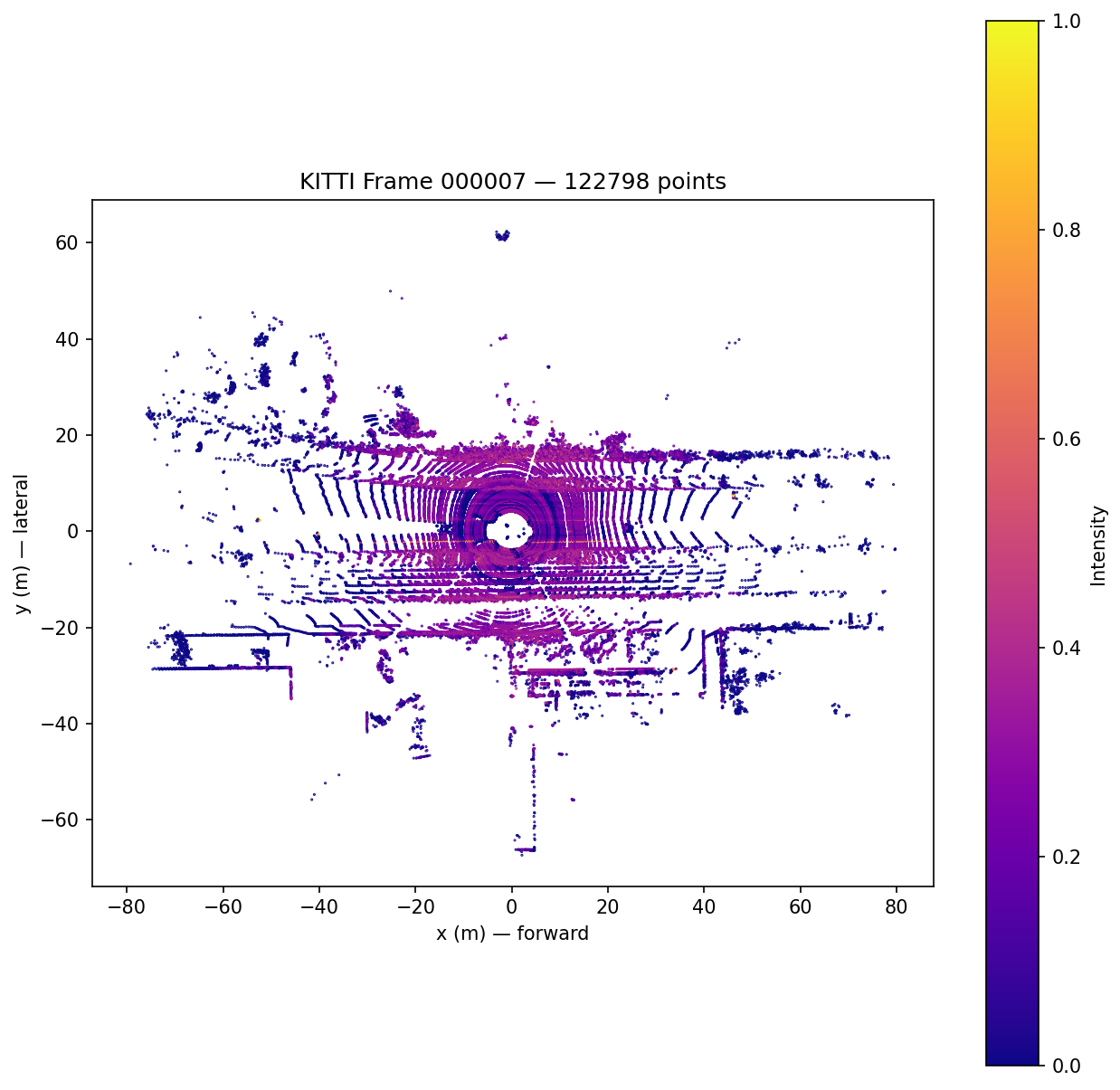
Fig. 1 KITTI frame 000007, 122,798 points, bird’s-eye view coloured by return intensity. This is the raw, unordered input the kernel consumes.
A PointPillars-style 3D object detector cannot read a raw LiDAR scan. The scan is an
unordered list of [x, y, z, intensity] points, and the network wants a dense grid of
fixed-size “pillars.” Voxelize is the CUDA kernel that does that conversion. It takes an
[N, 4] point cloud on the GPU and returns the three tensors PointPillars expects, a
[V, 32, 4] stack of per-pillar points, a [V, 3] list of pillar grid coordinates, and a
[V] count of points per pillar.
Due to this implementations use of a hash table, every point is an independent O(1) insert into
a hash table. This means a 25k-point frame and a 130k-point frame both take about a millisecond.
OpenPCDet’s reference voxel_generator scales roughly linearly with point count, so the gap between
them widens as frames get denser. This explains the large speedup values.
voxelize vs OpenPCDet voxel_generator (RTX 5060 Ti, uniform synthetic clouds)
| Points | voxelize | OpenPCDet | Speedup |
|---|---|---|---|
| 25k | 1.054 ms | 4.328 ms | 4.1× |
| 50k | 1.116 ms | 9.090 ms | 8.1× |
| 100k | 1.154 ms | 23.498 ms | 20.4× |
| 130k | 1.211 ms | 34.919 ms | 28.8× |
Tab. 1 Mean over 200 timed iterations after 20 warm-up iterations, torch.cuda.Event timing, inputs already resident on the GPU.
Design Decisions
The main struggle was that pillar assignment is the only part of this problem that is not trivially parallel. Computing a point’s grid cell is pure arithmetic, but grouping points that share a cell is a collision problem, and the naive solution (sort all points by cell ID, then segment) spends most of its time in the sort.
A hash table instead of a sort
Each point hashes its 2D grid ID into an open-addressing table held in global memory and
resolves collisions by linear probing. Claiming a cell is a single atomicCAS. A point that
finds its cell already claimed just reuses that slot. This turns “group N points” into N
independent constant-time operations with no global synchronisation, which is the real
reason the kernel is fast.
One thread per point
Thread i handles points[i] and nothing else. A point’s grid cell depends only on its own
coordinates, so there is no data to share between threads and no reason to tile or stage
anything in shared memory. Blocks are a flat 256 threads.
The hash slot is the output index
The kernel writes each pillar’s data at its hash slot h directly, and a post-pass compacts
the occupied slots into a dense array with a Thrust copy_if over the key table followed by a
gather kernel. The single counter disappears and the remaining atomics (atomicCAS to claim a slot,
atomicAdd on each pillar’s own point count) are spread across the table rather than serialised
on one address.
A fixed table, sized 8× the voxel budget
The table is 8 × max_voxels entries, allocated once per launch. Oversizing it keeps the
average probe length near one at the cost of memory and a cudaMemset to initialise it.
This creates some tradeoffs: the table size is fixed before the kernel runs, and the current
kernel assumes single-return LiDAR.
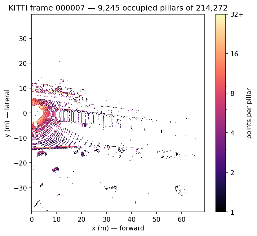
Fig. 2 Per-pillar point counts for frame 000007 on the 432 × 496 pillar grid (0.16 m cells), log colour scale. 9,245 of 214,272 pillars are occupied, densely near the sensor and sparsely at range. That non-uniform load is what the hash table has to absorb without a sort.
Implementation
Binning a point
The per-point device code checks for NaN/Inf, drops points outside the z-slab, computes
the cell with floorf (plain integer truncation rounds toward zero, which puts points just
below the origin in the wrong cell), and rejects anything outside the grid with a strict <
on the upper bound so a point exactly on x_max is excluded:
int cx = (int)floorf((x - x_min) / vx);
int cy = (int)floorf((y - y_min) / vy);
if (cx < 0 || cx >= grid_x) return -1;
if (cy < 0 || cy >= grid_y) return -1;
return cy * grid_x + cx;            // flattened voxel id
Claiming a pillar and packing points
int h = ((voxel_id % table_size) + table_size) % table_size;
while (true) {
    int old = atomicCAS(&hash_keys[h], -1, voxel_id);
    if (old == -1) {                       // the slot has been won
        coordinates[h * 3 + 0] = 0;        // z is always 0 for pillars
        coordinates[h * 3 + 1] = voxel_id / grid_x;
        coordinates[h * 3 + 2] = voxel_id % grid_x;
        break;
    }
    if (old == voxel_id) break;            // someone else already made this pillar
    h = (h + 1) % table_size;              // linear probe
}
int pt_idx = atomicAdd(&num_points_per_voxel[h], 1);
if (pt_idx >= max_points) return;          // pillar full, drop the point
for (int c = 0; c < C; c++)
    voxels[h * max_points * C + pt_idx * C + c] = points[idx * C + c];
The double modulo keeps the hash non-negative, atomicAdd returns each thread’s write
position inside the pillar, and dropping points past max_points matches the “keep the first
K” semantics of both the CPU reference and OpenPCDet. The key table is initialised to -1 in
one shot with cudaMemset(hash_keys, 0xFF, ...), since 0xFF bytes are -1 as a two’s
complement int32.
Compaction
After the kernel, the launcher walks the key table once:
thrust::copy_if(thrust::device,
                thrust::counting_iterator<int>(0),
                thrust::counting_iterator<int>(table_size),
                hash_keys_ptr,
                occupied_indices.begin(),
                [] __device__ (int k) { return k != -1; });
then a compact_kernel gathers those slots’ coordinates, counts, and point stacks into the
dense [V, ...] output tensors.
The PyTorch side
The op is a CUDAExtension built with -O3 --use_fast_math. The C++ wrapper does nothing but
TORCH_CHECK the dtype, contiguity, and device of every tensor and hand raw pointers to the
launcher. The Python entry point pre-allocates the output tensors, runs the call under
torch.no_grad() (voxelization has no gradient), and slices the outputs to the real pillar
count before returning.
voxelize latency vs point count (RTX 5060 Ti)
| Points | 25k | 50k | 100k | 130k |
|---|---|---|---|---|
| ms | 1.054 | 1.116 | 1.154 | 1.211 |
Tab. 2 A 5.2× increase in points costs 15% more time. The kernel is dominated by fixed launch and allocation overhead, not by the per-point work.
Results
Correctness is checked against two independent references. The first is a pure-NumPy
voxelize_cpu that uses a Python dict for pillar assignment, deliberately written in a
different language and style so that shared bugs are unlikely. The second is OpenPCDet’s own
voxel_generator. Because the hash table assigns slots in whatever order threads finish, both
comparisons sort by a flattened (z, y, x) key first, then assert the pillar sets and
per-pillar counts match. A handful of points land exactly on a cell boundary and can fall
either way under floating-point rounding, so boundary disagreements are allowed a small
tolerance.
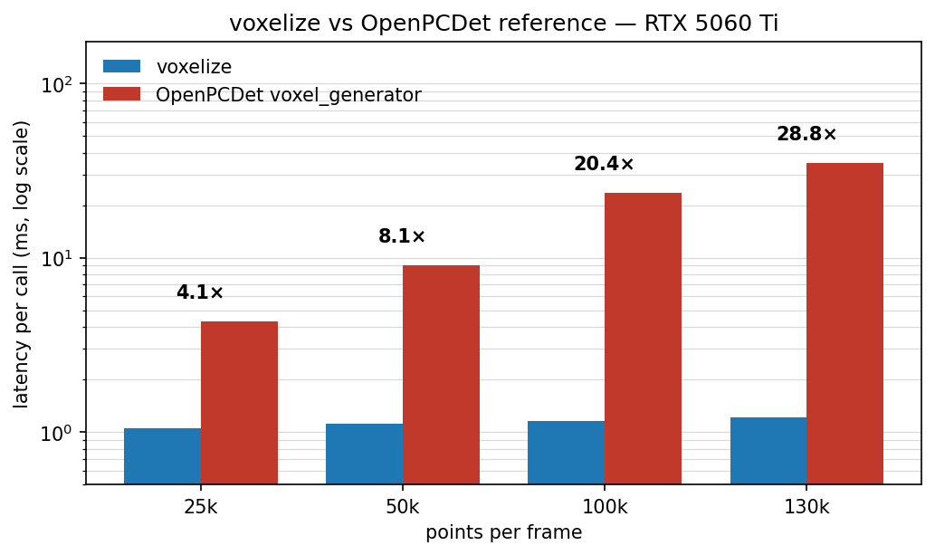
Fig. 3 voxelize vs OpenPCDet’s voxel_generator on uniform synthetic clouds, log scale. voxelize stays near 1 ms across the range; the reference op grows with point count, so the speedup climbs from 4.1× to 28.8×.
On five real KITTI frames the numbers hold up, and the speedup lands in a tighter band because real frames cluster near the sensor rather than filling the grid uniformly:
Real KITTI frames (RTX 5060 Ti)
| Frame | Points | voxelize | OpenPCDet | Speedup |
|---|---|---|---|---|
| 0 | 115,384 | 0.946 ms | 21.239 ms | 22.5× |
| 1 | 120,268 | 1.026 ms | 21.948 ms | 21.4× |
| 2 | 126,891 | 0.972 ms | 21.149 ms | 21.8× |
| 3 | 113,110 | 0.967 ms | 18.469 ms | 19.1× |
| 4 | 115,976 | 1.026 ms | 20.695 ms | 20.2× |
For scale, the NumPy reference that produced Fig. 1 and Fig. 2 takes 128 ms at 25k points and 534 ms at 130k. This ensures correctness and is not meant to be a baseline.
Limitations:
- this is measured against a single reference implementation on one GPU
- the hash table is sized statically at launch
- the synthetic benchmark uses a uniform distribution where real LiDAR is highly clustered, which is why the KITTI pass is reported separately
What’s Next?
- Profile with NSight Compute and apply the optimizations that it points to.