Talus
Rockfall Hazard Quantification for Alpine Routes — blog
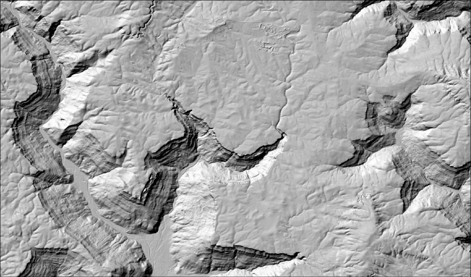
Fig. 1 Hillshade of Foster Falls, Tennessee, rendered from a USGS 3DEP 1/3 arc-second DEM (~10 m/cell).
Rockfall is one of the leading causes of death and serious injury in outdoor rock climbing and has no standardized or meaningful methods of detection or dissemination. Talus seeks to provide climbers with rockfall danger report by creating an end-to-end pipeline that turns a public elevation model into a concrete rockfall risk score for a specific wall
Talus ingests a USGS DEM and geology polygons, runs GPU-accelerated terrain analysis to find likely rockfall source zones, pulls temperature forecasts to compute freeze-thaw risk windows, and scores each route by its proximity to hazards uphill of it. Results are displayed on a map with source zone overlays and webhook alerts when risk crosses a predefined threshold.
The greatest engineering constraint here is scale. A single climbing area at 1/3 arc-second resolution is ~117 million cells, and every terrain derivative (slope, aspect, curvature, ruggedness) is a computation over every cell. On a single CPU thread that is multiple seconds per kernel although on a consumer GTX 1060 it is a few hundred milliseconds.
GPU vs. single-threaded CPU (GTX 1060 3GB, Foster Falls, 116.9M cells)
| Kernel | GPU | CPU | Speedup |
|---|---|---|---|
| Sobel slope/aspect | 569 ms | 6,041 ms | 10.6× |
| Plan/profile curvature | 565 ms | 1,180 ms | 2.1× |
| Terrain Ruggedness Index | 318 ms | 1,633 ms | 5.1× |
Design Decisions
The guiding design principle was to keep each concern in the language that fits it best and let a shared spatial database be the integration point.
Go microservices
The pipeline splits into four Go services: ingestion, GPU terrain preprocessing, hazard analysis, and an API gateway along with a standalone CUDA binary and one PostgreSQL + PostGIS database. Services talk over REST and hand off through the database.
| Service | Language | Responsibility |
|---|---|---|
| S1 — Ingestion | Go | GeoTIFF parse, GPX ingest, geology polygon ingest |
| S2 — Terrain | Go + CUDA subprocess | GPU terrain derivatives, source zone detection |
| S4 — Hazard | Go | Proximity risk scoring, freeze-thaw compute, webhooks |
| S5 — Gateway | Go + Leaflet.js | REST API, static dashboard |
| PostgreSQL | SQL + PostGIS | Shared persistent store, spatial queries |
CUDA as a subprocess
S2 invokes the CUDA terrain binary as a child process and exchanges data through raster files on a shared Docker volume.
PostGIS for the proximity model
Since risk scoring is a spatial question (which source zones sit
uphill and within N meters of this route?), it belongs in the database.
ST_DWithin against source zone centroids does the proximity query directly,
and the route/derivative/analysis tables stay spatially indexed rather than
being pulled into application memory.
USGS 3DEP ──► S1 Ingestion (Go) ──► S2 Terrain Preprocessing (Go)
                                              │
                                       CUDA Binary (C/CUDA)
                                       Sobel · Curvature · TRI
                                              │
NOAA NOMADS ──► S4 Hazard Analysis (Go) ◄────┘
                        │
                        ▼
               S5 API Gateway (Go) ──► Browser / Mobile Client
                        │
               PostgreSQL + PostGIS
Fig. 2 Data flow. External inputs enter through S1, terrain derivatives are computed by the CUDA subprocess under S2, and S4 adds weather to score routes. S5 is what the client talks to.
Implementation
The Sobel slope/aspect kernel
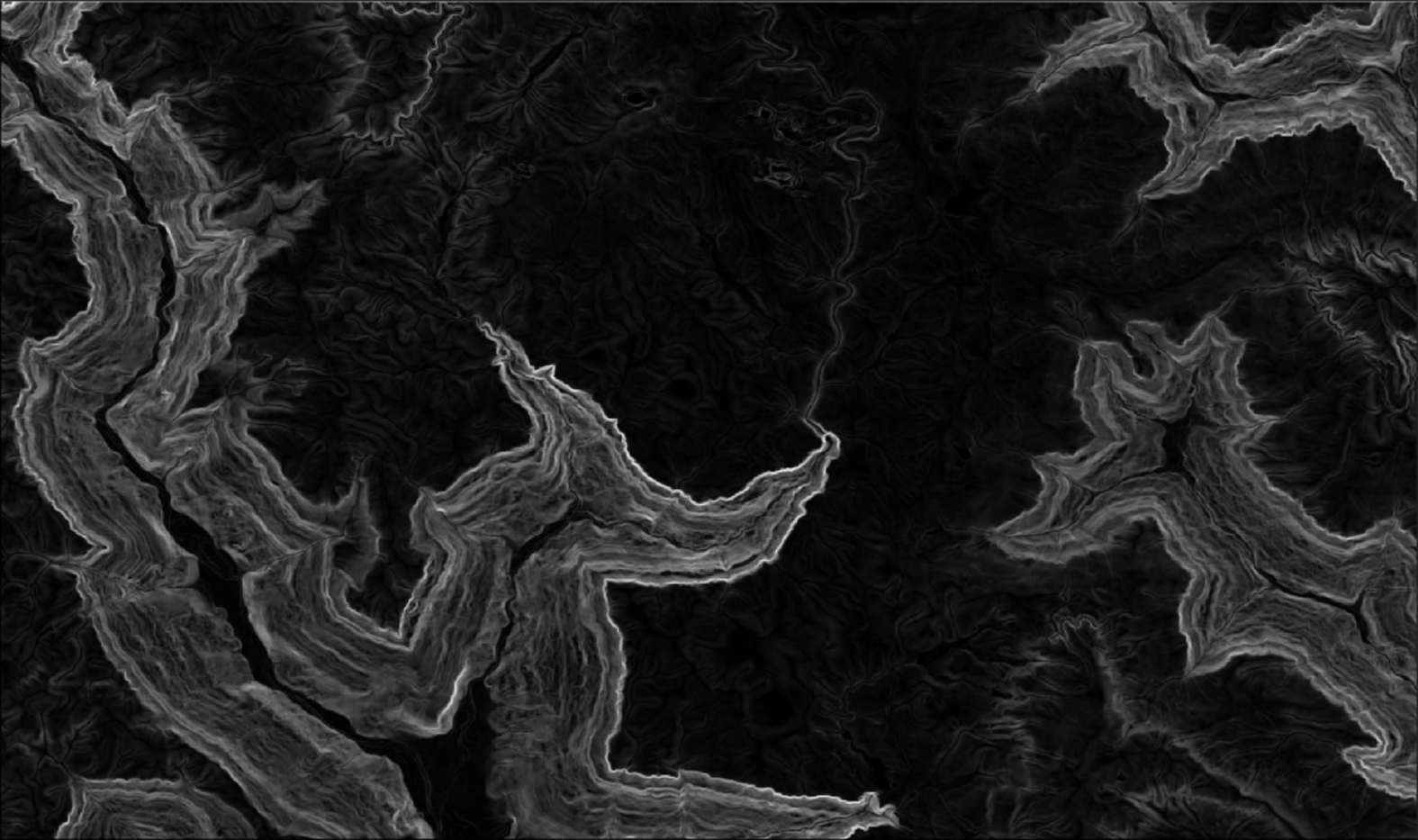
Slope and aspect are both derrived from the elevation gradient and estimated per cell with a 3×3 Sobel convolution over the 8 neighbors. The horizontal and vertical neighbors are weighted twice as heavily as the diagonals, which sit √2 farther from the center:
Sobel X (E–W gradient)     Sobel Y (N–S gradient)
-1  0  +1                    +1  +2  +1
-2  0  +2                     0   0   0
-1  0  +1                    -1  -2  -1
From the two gradient components gx and gy:
slope  = atan( sqrt(gx² + gy²) / cell_size ) × (180 / π)
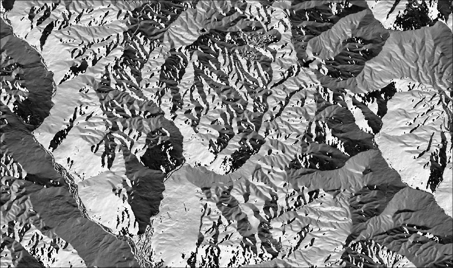
aspect = 90 - atan2(gy, -gx) × (180 / π)
The atan2 term returns −π to π with east at 0. Subtracting from 90° rotates it
into a compass bearing with north at 0, and any remaining negative angles get
360° added to wrap them positive.
Curvature and ruggedness
Plan/profile curvature (second derivatives of elevation) and the Terrain Ruggedness Index (mean absolute elevation difference to neighbors) use the same one-thread-per-cell pattern but have lower arithmetic intensity, which explains why their speedups land at 2–5× rather than 10×.
Freeze-thaw windows
S4 pulls NOAA HRRR temperature forecasts for the area’s elevation band and computes freeze-thaw cycles. Aspect determines when a face is sun-warmed, so a west-facing wall and an east-facing wall get different risk timelines from the same forecast.
Proximity risk scoring
The final score for a route is a product of the terms that actually move rockfall hazard:
risk = proximity × slope × freeze_thaw
proximity comes from an ST_DWithin query for source zone centroids uphill
of the route, slope from the steepest contributing source cell, and
freeze_thaw from the current window. When the score crosses a configured
threshold, S4 fires a webhook.
Results
The benchmark numbers above are queried directly from the terrain_metrics
table after a real end-to-end run (gpu_time_ms, cpu_time_ms, and
throughput_mcps) are recorded by the CUDA binary. The CPU baseline is
a single-threaded implementation of the same computation, so the speedup
reflects the GPU against one core, not against an optimized multi-threaded
CPU version.
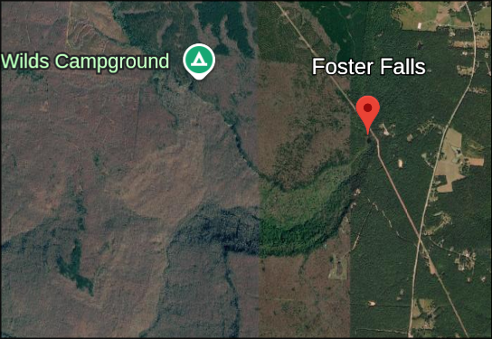
Fig. 4 Reference imagery for the same extent. The GPU-derived cliff bands in Fig. 3 line up with the visible exposed rock here
What’s Next?
A continuation of this work would likely explore:
- Monte Carlo simulations for rock fall to find probable rock landing zones.
- A atmospheric model for freeze-thaw instead of a single elevation band.